MATLAB & Simulink

In our digital mixer, we want to utilize various types of filters to control parameters such as the volume of specific frequency bands or to cut off part of the frequency spectrum. To create these filters, we used MATLAB, Simulink and the HDL Coder from MATLAB to generate VHDL code as a foundation for further development.

Low & High Pass Filter

As mentioned in the introduction to this chapter, we want to able to cut off part of the frequency spectrum from the input sources of our digital mixer. To achieve this, we will employ both low-pass and high-pass filters.

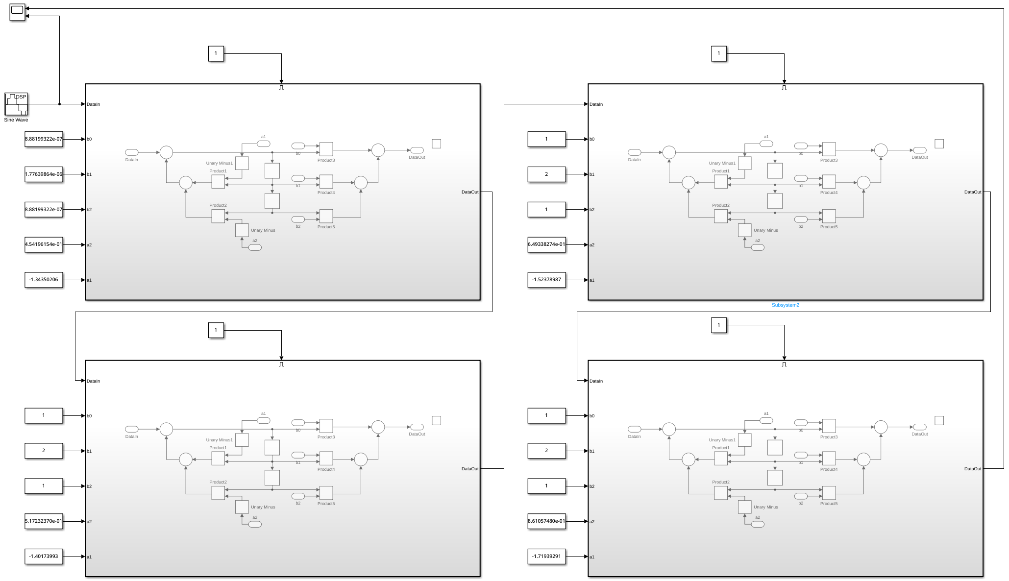
In Simulink, we designed an 8th order low-pass & high-pass filter by using a Cascade of four Direct Form 2 Digital Biquad Filters.

• Top view of the low-pass Filter

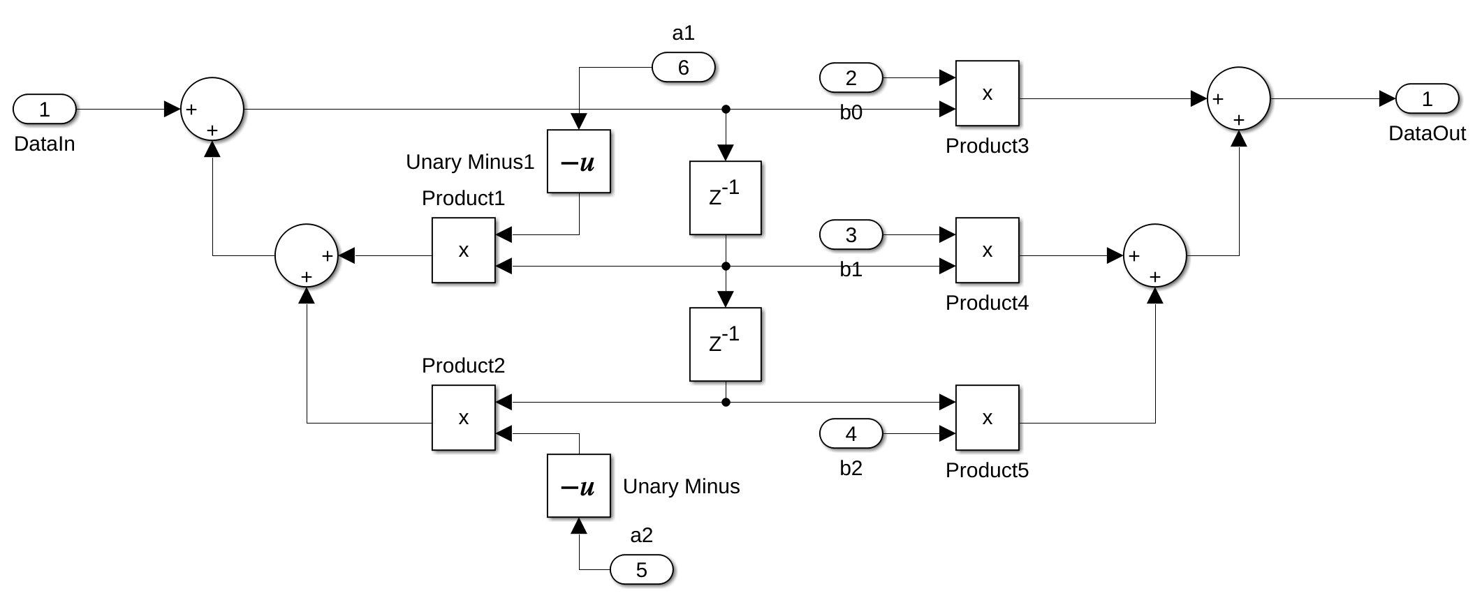
• Direct Form 2 Digital Biquad Filter

The Simulink files for the low-pass & high-pass Filters can be found in the Git Repo.

A biquad filter is a second order filter containing two poles and two zeros. In the Z-domain, the transfer function for this type of filter is the ratio of two quadratic functions:

\[ H(z)=\frac{b_0+b_1z^{-1}+b_2z^{-2}}{a_0+a_1z^{-1}+a_2z^{-2}} \]

The filter coefficients are often normalized so that \(a_0 = 1\), which is also the case in the Python library we use to generate these coefficients. The updated transfer function, shown below, is the same as the one implemented in Simulink, as illustrated in the image above:

\[ H(z)=\frac{b_0+b_1z^{-1}+b_2z^{-2}}{1+a_1z^{-1}+a_2z^{-2}} \]

We are using a Python library called SciPy to generate the coëfficients for these filters. To be able to work with SciPy, we need to install the following package:

pip3 install scipy

This is the script to get the coëfficients for the low-pass filter:

from scipy import signal
from scipy.signal import sos2tf

N = 8 # filter order
wn = 3000/(48000/2) # natural frequency between 0 and 1
sos = signal.iirfilter(N, wn, btype='lowpass', output = 'sos', ftype='butter')

print(sos)

You can use the same code for generating the coëfficients for the high-pass filter by changing btype to highpass.

To estimate the time required to generate these coefficients, we created a simple script that generates coefficients for a thousand low-pass filters with varying cut-off frequencies.

from scipy import signal
import time
import numpy as np

N = 8  # filter order

execution_times = []

for i in range(1000):
    start_time = time.time()

    wn = 3*(i+1) / (48000 / 2)  # natural frequency between 0 and 1
    sos = signal.iirfilter(N, wn, btype='lowpass', output='sos', ftype='butter')

    end_time = time.time()
    execution_times.append(end_time - start_time)

# Calculate statistics
average_time = np.mean(execution_times)
min_time = np.min(execution_times)
max_time = np.max(execution_times)

print(average_time*1000)
print(min_time*1000)
print(max_time*1000)

Here are the results obtained from running the script:

• Average execution time: 0.88 milliseconds
• Minimum execution time: 0.74 milliseconds
• Maximum execution time: 1.78 milliseconds

Info

The filter coefficients generated by this Python script are too small when implementing an 8th-order Low or High Pass filter, leading to significant errors during conversion to fixed-point representation with 23-bit precision. Therefore, we decided to use a 2nd-order Low Pass filter and a 4th-order High Pass filter instead.

Shelving Filters

Our goal is to control the gain of the low, mid, and high-frequency ranges of the input sources. To achieve this, we aim to design a filter capable of amplifying or attenuating the gain in the low (<200 Hz), mid (200 Hz to <2 kHz), and high (≥2 kHz) frequency bands. The filter type we've selected for this purpose is the shelving filter. Shelving filters are particularly well-suited for this task, as they allow for precise gain adjustments within a specific frequency band while leaving the rest of the frequency spectrum unaffected.

We have reviewed several research papers on designing these filters digitally and have selected this particular paper as our primary source of information.

Low Shelf

Following is a brief summary of all the variables, and their meanings, that you need to know to calculate the coëfficients for the Low Shelf version of these type of filters.

\[ \alpha_m=\left(\frac{1}{2}-\frac{2m-1}{2M}\right)\pi \]

\[ c_m=\cos(a_m) \]

\[ V=\sqrt[M]{g}-1 \]

\[ K=\tan\left(\frac{\Omega_B}{2}\right) \]

• M is the filter order
• m is the m-th second order section of the filter
• \(a_m\) is the angle of the pole and zero of the m-th section
• g is the amplification/attenuation of the filter in V/V
• \(\Omega_B\) is the filter bandwidth in radians per sample

\(\Omega_B\) can be calculated usting the following formula: $$\Omega_B = \frac{f_{band}}{f_{\frac{s}{2}}}\pi$$

We are using the same biquad filters to implement the shelving filters. The transfer function given in the paper cannot be directly mapped to the \(a_0\), \(a_1\), \(a_2\), \(b_0\), \(b_1\) and \(a_2\) variables. After some calculation, this is the result:

\[ a_0 = K^2 + 2K\cdot c_m + 1 \]

\[ a_1 = 2K^2-2 \]

\[ a_2 = K^2 - 2K\cdot c_m + 1 \]

\[ b_0 = K^2(V^2+2V+1) + 2K\cdot c_m(V+1) +1 \]

\[ b_1 = 2K^2(V^2+2V+1)-2 \]

\[ b_0 = K^2(V^2+2V+1) - 2K\cdot c_m(V+1) +1 \]

High Shelf

To calculate the High Shelf filter, follow the same procedure as for the Low Shelf filter. However, to achieve a High Shelf response, you need to negate the \(a_1\) and \(b_1\) coefficients.

Band Shelf

To create a Band Shelf filter, the input signal is first amplified or attenuated to the desired gain. Then, a Low Shelf filter is cascaded with a High Shelf filter to amplify or attenuate the low and high frequency bands, matching it to the level of the original input signal.

MATLAB Simulations

%% Low Shelf 4th order

K = 0.01964;   % 100Hz Bandwidth
V = -0.250106;    % -10dB

% Filter 1
Cm = 0.382683;

% Filter coëfficients
a0 = 1 + 2*K*Cm + K^2
a1 = 2*K^2 - 2
a2 = 1 - 2*K*Cm + K^2
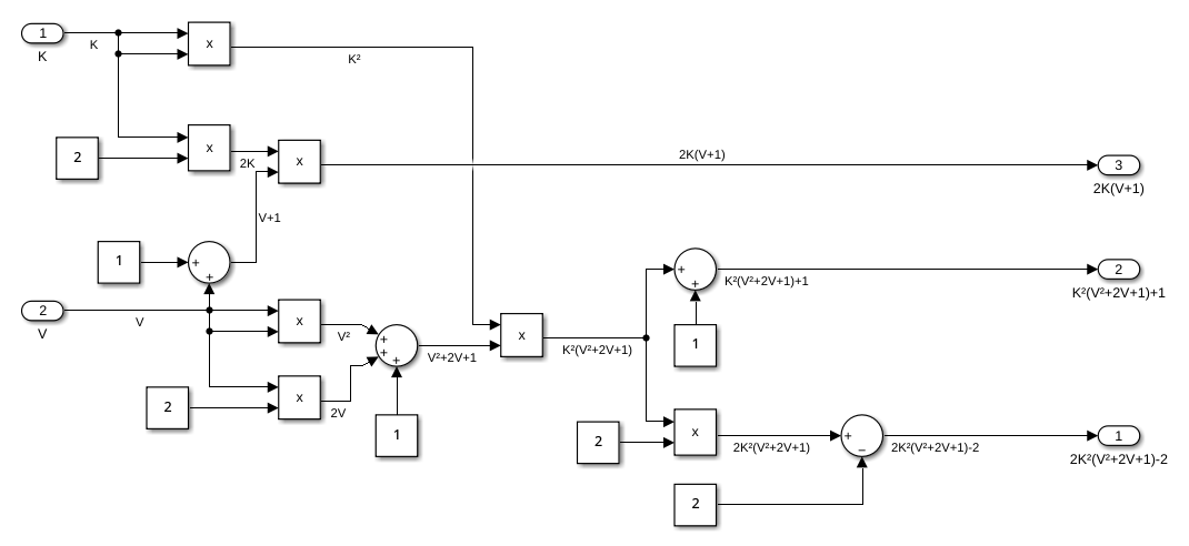
b0 = K^2*(V^2 + 2*V +1) + 2*K*Cm*(V+1) + 1
b1 = 2*K^2*(V^2 + 2*V +1) -2
b2 = K^2*(V^2 + 2*V +1) - 2*K*Cm*(V+1) + 1

% Normalization
b0 = b0/a0
b1 = b1/a0
b2 = b2/a0
a1 = a1/a0
a2 = a2/a0
a0 = a0/a0

ts = 1/48000;
z = tf('z',ts);
ls1 = (b0 + b1*z^(-1) + b2*z^(-2))/(a0 + a1*z^(-1) + a2*z^(-2))

% Filter 2
Cm = 0.92388;

% Filter coëfficients
a0 = 1 + 2*K*Cm + K^2
a1 = 2*K^2 - 2
a2 = 1 - 2*K*Cm + K^2
b0 = K^2*(V^2 + 2*V +1) + 2*K*Cm*(V+1) + 1
b1 = 2*K^2*(V^2 + 2*V +1) -2
b2 = K^2*(V^2 + 2*V +1) - 2*K*Cm*(V+1) + 1

% Normalization
b0 = b0/a0
b1 = b1/a0
b2 = b2/a0
a1 = a1/a0
a2 = a2/a0
a0 = a0/a0

ts = 1/48000;
z = tf('z',ts);
ls2 = (b0 + b1*z^(-1) + b2*z^(-2))/(a0 + a1*z^(-1) + a2*z^(-2))

ls4 = ls1 * ls2
bp = bodeplot(ls4);
bp.FrequencyUnit = "Hz";
bp.PhaseVisible = "off";

%% High Shelf 4th order

K = 2.4142;     % 18kHz Bandwidth
V = 0.154782;    % +5dB

% Filter 1
Cm = 0.382683;

% Filter coëfficients
a0 = 1 + 2*K*Cm + K^2
a1 = 2*K^2 - 2
a2 = 1 - 2*K*Cm + K^2
b0 = K^2*(V^2 + 2*V +1) + 2*K*Cm*(V+1) + 1
b1 = 2*K^2*(V^2 + 2*V +1) -2
b2 = K^2*(V^2 + 2*V +1) - 2*K*Cm*(V+1) + 1

% Normalization
b0 = b0/a0
b1 = b1/a0
b2 = b2/a0
a1 = a1/a0
a2 = a2/a0
a0 = a0/a0

ts = 1/48000;
z = tf('z',ts);
hs1 = (b0 + b1*(-z)^(-1) + b2*(-z)^(-2))/(a0 + a1*(-z)^(-1) + a2*(-z)^(-2))

% Filter 2
Cm = 0.92388;

% Filter coëfficients
a0 = 1 + 2*K*Cm + K^2
a1 = 2*K^2 - 2
a2 = 1 - 2*K*Cm + K^2
b0 = K^2*(V^2 + 2*V +1) + 2*K*Cm*(V+1) + 1
b1 = 2*K^2*(V^2 + 2*V +1) -2
b2 = K^2*(V^2 + 2*V +1) - 2*K*Cm*(V+1) + 1

% Normalization
b0 = b0/a0
b1 = b1/a0
b2 = b2/a0
a1 = a1/a0
a2 = a2/a0
a0 = a0/a0

ts = 1/48000;
z = tf('z',ts);
hs2 = (b0 + b1*(-z)^(-1) + b2*(-z)^(-2))/(a0 + a1*(-z)^(-1) + a2*(-z)^(-2))

hs4 = hs1 * hs2
bp = bodeplot(hs4);
bp.FrequencyUnit = "Hz";
bp.PhaseVisible = "off";

%% Band Shelf 8th order

K = 0.013091;   % 100Hz Bandwidth
V = 1.11349; %+26dB

% Volume
ap = 0.0501*z^(0); %-26dB

% Filter 1 (Low Shelf)
Cm = 0.382683;

% Filter coëfficients
a0 = 1 + 2*K*Cm + K^2
a1 = 2*K^2 - 2
a2 = 1 - 2*K*Cm + K^2
b0 = K^2*(V^2 + 2*V +1) + 2*K*Cm*(V+1) + 1
b1 = 2*K^2*(V^2 + 2*V +1) -2
b2 = K^2*(V^2 + 2*V +1) - 2*K*Cm*(V+1) + 1

% Normalization
b0 = b0/a0
b1 = b1/a0
b2 = b2/a0
a1 = a1/a0
a2 = a2/a0
a0 = a0/a0

ts = 1/48000;
z = tf('z',ts);
bs1 = (b0 + b1*z^(-1) + b2*z^(-2))/(a0 + a1*z^(-1) + a2*z^(-2))

% Filter 2 (Low Shelf)
Cm = 0.92388;

% Filter coëfficients
a0 = 1 + 2*K*Cm + K^2
a1 = 2*K^2 - 2
a2 = 1 - 2*K*Cm + K^2
b0 = K^2*(V^2 + 2*V +1) + 2*K*Cm*(V+1) + 1
b1 = 2*K^2*(V^2 + 2*V +1) -2
b2 = K^2*(V^2 + 2*V +1) - 2*K*Cm*(V+1) + 1

% Normalization
b0 = b0/a0
b1 = b1/a0
b2 = b2/a0
a1 = a1/a0
a2 = a2/a0
a0 = a0/a0

ts = 1/48000;
z = tf('z',ts);
bs2 = (b0 + b1*z^(-1) + b2*z^(-2))/(a0 + a1*z^(-1) + a2*z^(-2))


K = 2.4142;     % 18kHz Bandwidth

% Filter 3 (High Shelf)
Cm = 0.382683;

% Filter coëfficients
a0 = 1 + 2*K*Cm + K^2
a1 = 2*K^2 - 2
a2 = 1 - 2*K*Cm + K^2
b0 = K^2*(V^2 + 2*V +1) + 2*K*Cm*(V+1) + 1
b1 = 2*K^2*(V^2 + 2*V +1) -2
b2 = K^2*(V^2 + 2*V +1) - 2*K*Cm*(V+1) + 1

% Normalization
b0 = b0/a0
b1 = b1/a0
b2 = b2/a0
a1 = a1/a0
a2 = a2/a0
a0 = a0/a0

ts = 1/48000;
z = tf('z',ts);
bs3 = (b0 + b1*(-z)^(-1) + b2*(-z)^(-2))/(a0 + a1*(-z)^(-1) + a2*(-z)^(-2))

% Filter 4 (High Shelf)
Cm = 0.92388;

% Filter coëfficients
a0 = 1 + 2*K*Cm + K^2
a1 = 2*K^2 - 2
a2 = 1 - 2*K*Cm + K^2
b0 = K^2*(V^2 + 2*V +1) + 2*K*Cm*(V+1) + 1
b1 = 2*K^2*(V^2 + 2*V +1) -2
b2 = K^2*(V^2 + 2*V +1) - 2*K*Cm*(V+1) + 1

% Normalization
b0 = b0/a0
b1 = b1/a0
b2 = b2/a0
a1 = a1/a0
a2 = a2/a0
a0 = a0/a0

ts = 1/48000;
z = tf('z',ts);
bs4 = (b0 + b1*(-z)^(-1) + b2*(-z)^(-2))/(a0 + a1*(-z)^(-1) + a2*(-z)^(-2))


bs8 = bs1 * bs2 * bs3 * bs4
bp = bodeplot(bs8);
bp.FrequencyUnit = "Hz";
bp.PhaseVisible = "off";

bs8 = bs8 * ap;
bp = bodeplot(bs8);
bp.FrequencyUnit = "Hz";
bp.PhaseVisible = "off";

We did some MATLAB Simulations to verify whether the shelving filters work as intended.

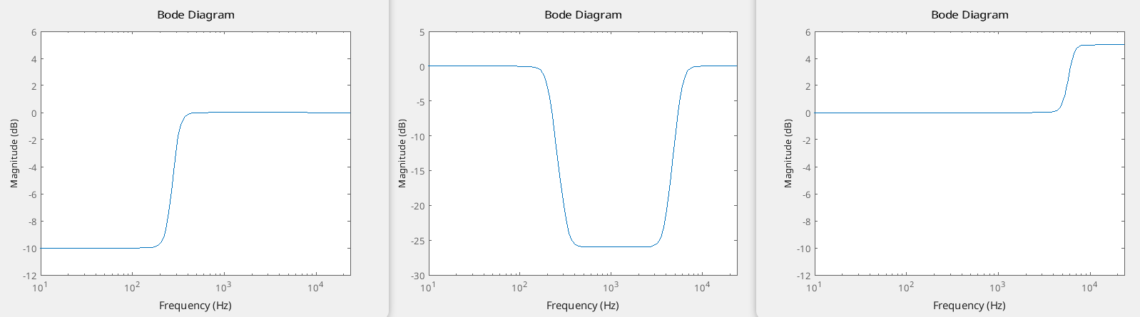
The image above illustrates, from left to right: a Low Shelf filter with a gain of -10dB and a bandwidth of 300Hz, a Band Shelf filter with a gain of -26dB and a bandwidth of 6kHz, and a High Shelf filter with a gain of +5dB and a bandwidth of 18kHz.

Simulink

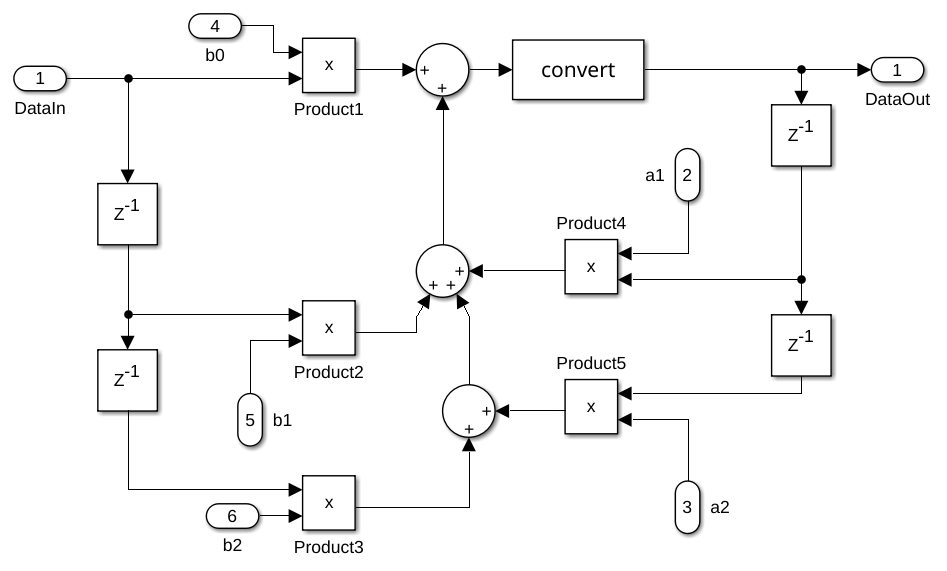
We used the same Direct Form 2 Digital Biquad Filter in Simulink to test out the shelving filters. However, this fitler overflowed almost instantly. This is actually a disadvantage of the Direct Form 2 stucture, it can cause numbers to get too large to handle (arithmetic overflow) when using a certain combination of filter coëfficients.

So, we switched to the Direct Form 1 Digital Biquad Filter as shown in the image below.

Info

Because of the overflow issue, we also switched the Low and High pass filter to the Direct Form 1 Digital Biquad Filter structure. This ensures that all the filters we develop share the same structure, allowing us to implement a single, unified filter design in VHDL.

Rather than pre-calculating the filter coefficients, we incorporated the formulas for calculating them directly within Simulink. This approach allows us to convert the Simulink model into functional HDL code.

Info

However, calculating the coefficients for the required 8 biquad filters — 4 for the band shelf, 2 for the low shelf, and 2 for the high shelf — demands a significant number of DSP slices. The Ultra96-V2 lacks sufficient DSP slices to handle all these calculations, causing Vivado to use regular logic slices instead. This led to extremely high logic and net delays, exceeding 100 ns. To address this issue, we decided to offload the coefficient calculations to the Processing System (PS) instead of performing them on the Programmable Logic (PL).

This was the result of simulating the Low Shelf filter with a bandwidth of 400Hz and a gain of +5dB when passing a sine wave of 100Hz and 400Hs through the filter.

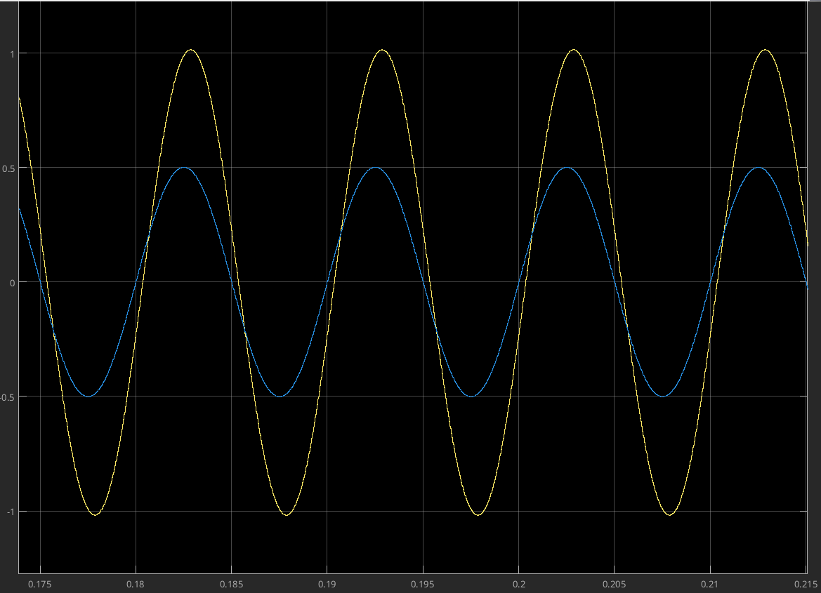
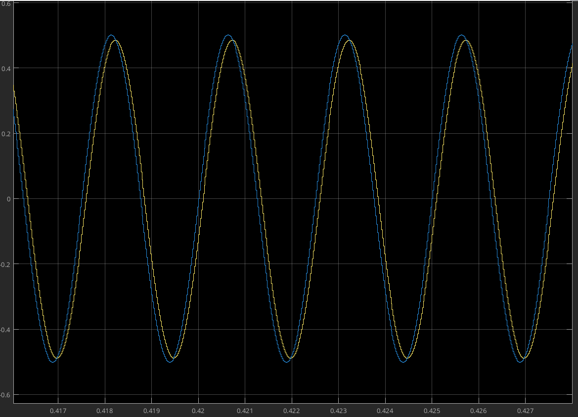
We can conclude that this filter works as intended, as it amplifies the sine at 100Hz and doesn't change the sine wave at 400Hz.

Audio Effects

We also want to add some audio effects to the audio pipeline. The chosen effects are saturation, echo and ring modulation. We tested the saturation and echo first in Simulink before implementing it in VHDL.

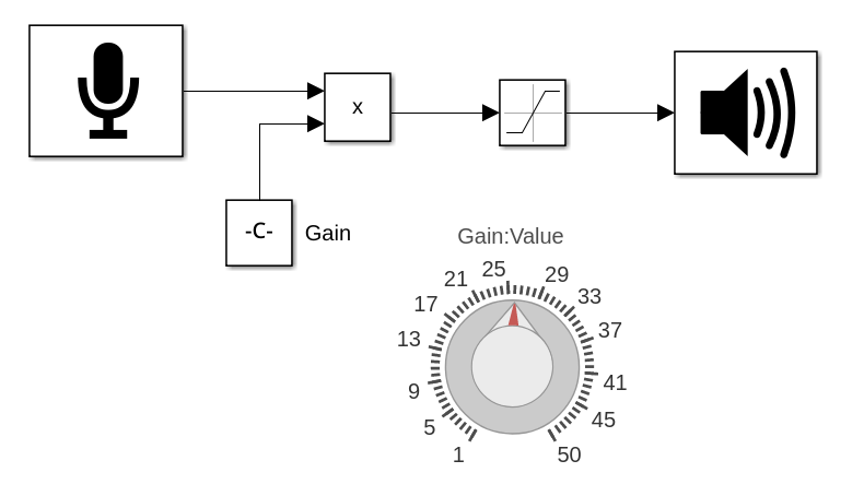
Saturation

The saturation audio effect is a type of signal processing that emulates the natural distortion and harmonic enhancement produced when an analog audio signal is pushed beyond its normal operating range. This effect occurs in analog devices such as tape recorders, tube amplifiers, or analog mixing consoles. In digital audio, saturation is used creatively to add warmth, color, and character to sound.It adds more aggressive harmonics and distortion, often used for a gritty sound.

Echo

The echo audio effect is a sound processing technique that creates a repetition of the original sound after a delay, mimicking the natural phenomenon of sound reflecting off surfaces. Echo effects are widely used in music production, sound design, and audio engineering to add depth, space, and a sense of atmosphere to audio.

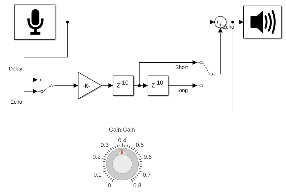
The simulations for the saturation and echo effects can be found in the Git Repo.

Ring Modulation

The ring modulation audio effect is a sound processing technique where two signals—typically referred to as the carrier and the modulator—are multiplied together, producing a new sound that consists of the sum and difference of their frequencies. This effect is widely used in music production, particularly in experimental and electronic music, as well as in sound design for its unique, metallic, and often inharmonic qualities.